Example 1:
- Suppose we have a list of products and their prices (A1 tem D18), and we want to find the prices (G2 tem G5) of the products (F2 tem F5). This example can be easily solved with XLOOKUP, unlike VLOOKUP.
= XLOOKUP (F2; D1: D18; B1: B18)
In this formula, Product Name (F2) is the value we want to search, D2: D18 is the range in which we want to search, and B2: B18 is the range in which we want to find the price. This will retrieve the price of the product based on the product name.

Example 2:
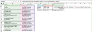
Another useful feature of XLOOKUP is that it can search based on multiple criteria (use the ‘&‘ or ampersand sign for this). For example, if we have a list of customers and orders and we want to find on which date a specific customer ordered a specific product, we can use the following formula:
= XLOOKUP ($G2&$H2; $D$2:$D$20&$B$2:$B$20; $C$2:$C$20; “wrong date or name”;0)

In this formula, G2 and H2 are the values we want to search (customer name and product), D2:D20 and C2:C20 are the ranges in which we want to search (customer name and product), and C2:C20 is the range in which we want to find the date. This will retrieve the date of the customer’s order for the specific product.
Tip:
Note that in the fourth field of the XLOOKUP, we can specify a text when the searched value can’t be found. It now reads “wrong product or name” whereas otherwise there would be an error message via VLOOKUP (NA). In the old VLOOKUP, we had to nest the additional function IFERROR. So through XLOOKUP, this is simply no longer necessary.
XLOOKUP is a very useful new feature that makes it easier to search and find data in Excel. Because of its versatility, it is definitely worth learning how to use it.